A Deep Dive into A/B Testing Fundamentals

Acme Corporation sells widgets. The new model, Widget K, has been highlighted on the front page of the company’s website. It’s a top-of-page banner-style image and the first thing you see when you visit the site. However, despite high traffic to the site, Widget K is not selling as well as anticipated. Let’s solve this problem with A/B testing.

Sally, the marketing manager, has come up with a new layout for a banner image that she thinks will result in a better click-through rate (CTR) and comes to you for advice on how to proceed. If this new Version B of the banner image is actually performing worse, she would like to discontinue its use as soon as possible.

Note: this article assumes that you understand the Central Limit Theorem, hypothesis testing and sampling distributions.

The Concept

In order to test the performance of the original Version A of the banner image against the new Version B, we will randomly serve both versions to website visitors. Over the course of the experiment, we’ll randomly select A or B with equal probability to maintain a fairly balanced dataset with respect to the number of visitors served one version versus the other. As you will see shortly, this condition will help to simplify some initial calculations that we’ll perform before we start the experiment. Here are some things that would be beneficial for Sally to know even before you start any experiment.

	Sample size: The number of visitors that we'll need in order to determine if there is a difference in performance between the two versions that is significant (and not just due to random chance).
	Statistical power: What our chances are that we'll discover a difference, if there is indeed a performance difference that can be attributed to one of the two versions.
	Experiment duration: Based on number of visitors needed for the experiment, some idea of how long we'd need to run the experiment.
	Early stopping: That there is a possibility of ending the experiment early, if there is a strong enough signal to detect.

The Challenge

Suppose you were playing a video game with a friend and he scored 560 points while you scored 559. Assuming that scoring one point is as easy as, say, collecting a coin by running into it, would you conclude that he’s better at the game than you? Probably not, since the scores were almost the same. It could have gone either way, right? What if you played 10 games and every time, he happened to beat you by one point? At this point, even though he’s consistently doing better, it’s not by much and you may still say that your skill levels are about the same. What if after 1000 games, he’s won every single game by one point? At this point, you’d have to admit that he’s doing something consistently better, right?

Now let’s say you challenged another friend and this time she scored 1000 points while you only scored 580? You thought it was a fluke so you played two more games. Each time, she beat you by over 400 points? Do you feel you need to play any more games to determine who the better player is?

Based on the two scenarios above, here are some reasonable hypotheses.

Detecting small differences is harder than detecting large differences.
When the difference is small, there’s a higher possibility that it was just due to random chance than when the difference is large.
For detecting small differences, we need more data than when detecting large ones.
By running experiments longer and collecting more data, we can be more certain of the differences that we detect.
Conversely, larger differences are easier to detect, require less data to convince us and generally lead to shorter experiments.

Statistical Power

At the heart of A/B testing is the concept of the statistical power of an experiment. For the two versions of the Widget K banner images, we’re interested in knowing which version leads to a better CTR (proportion of impressions that resulted in a click-through), so we’re conducting hypothesis testing for the difference between proportions. (If we were measuring some average such as the average time the user stays on a web page, we’d use hypothesis testing for the difference between means.)

Let’s say that Sally gave you the following information:

The current CTR for the version currently on the website is approximately 0.5%.
She’s hoping that the new version will increase the CTR to 1%.
A false positive rate of 5% is acceptable for hypothesis testing.

So we’re trying to detect a 0.5% increase in CTR. This difference is referred to as an effect and the size of the difference is called the effect size. What do we need to do in order to detect this effect?

The Null Model

As with every hypothesis test, we need a null hypothesis \((H_0)\). In our case, our null hypothesis would be that “there is no difference in CTR between version A and B.” We then set out to find evidence that leads us to reject \(H_0\) or, if we fail to gather such evidence, fail to reject it. We can draw a model to represent \(H_0\) in the form of a Normal distribution. We can use a Normal distribution since we are modelling the sampling distribution of the difference between proportions. We know that this Normal distribution should be centred at zero since \(H_0\) states that there is no difference between the proportions. But what standard deviation do we use?

Population vs Sample

Let’s sidetrack for a moment to clarify population vs. sample in the context of website data. It’s easy to think that all the data collected by your webserver represent the population data but from a statistical point of view, you’ve only collected data that represent one possible reality. In other words, if you were to clean out all your data and start over, you’d simply have another sample.

Since we are dealing with a sample, we need to determine the standard error of the difference between proportions for versions A and B.

SE of the Difference between Proportions	SE of the Difference between Means
\(SE = \sqrt{\dfrac{\hat{p}_a \hat{q}_a}{n_a} + \dfrac{\hat{p}_b \hat{q}_b}{n_b}} \)	\(SE = \sqrt{\dfrac{s_a^2}{n_a} + \dfrac{s_b^2}{n_b}} \)
\(\hat{p}_a\), CTR for Version A \(\hat{p}_b\), CTR for Version B \(\hat{q}_a = 1 - \hat{p}_a\) \(\hat{q}_b = 1 - \hat{p}_b\) \(n_a\), sample size for Version A \(n_b\), sample size for Version B	\(s_a\), sample std. dev. for Version A \(s_b\), sample std. dev. for Version B \(n_a\), sample size for Version A \(n_b\), sample size for Version B

We know the current CTR for Version A is 0.005 and we would like the CTR for Version B to increase a half of a percent to 0.01.

\(\hat{p}_a=0.005\)
\(\hat{p}_b=0.01\)
\(\hat{q}_a=1-\hat{p}_a=1-0.005=0.995\)
\(\hat{q}_b=1-\hat{p}_b=1-0.01=0.99\)

Now, let’s assume we had randomly served each version 1000 times to website visitors by assigning each visitor randomly to either version A or version B with equal probability. We can now calculate the standard error of the difference between proportions (for 1000 visitors in each group).

\[ SE = \sqrt{\dfrac{\hat{p}_a \hat{q}_a}{n_a} + \dfrac{\hat{p}_b \hat{q}_b}{n_b}} = \sqrt{\dfrac{\hat{p}_a \hat{q}_a + \hat{p}_b \hat{q}_b}{n}} \]

But wait! If the null hypothesis is true, we’re saying that there is no significant difference in CTR, so we’ll use a pooled standard error instead. Given that both groups have the same number of observations, we can replace the single proportion with an average of the two.

\[ SE_{pooled} = \sqrt{2 \times \frac{\hat{p}_{pooled}\hat{q}_{pooled}}{n}} = \sqrt{\frac{2}{n} \times \frac{\hat{p}_a+\hat{p}_b}{2} \times \frac{(1-\hat{p}_a) + (1-\hat{p}_b)}{2}} \] \[= \sqrt{\frac{1}{n}} \space \sqrt{(\hat{p}_a+\hat{p}_b)\left(1-\frac{\hat{p}_a+\hat{p}_b}{2}\right)}\]

The \(\sqrt\frac{1}{n}\) has been factored out for clarity and will help with the math later on as we derive the power formula used by one of the R functions from the stats package.

Using a standard significance level \((\alpha)\) of 0.05,

> alpha <- 0.05
> p_a <- 0.005; q_a <- 1 - p_a
> p_b <- 0.010; q_b <- 1 - p_b
> n <- 1000
> SE_pooled <- sqrt(1/n) * sqrt((p_a + p_b) * (1 - (p_a + p_b) / 2))
> critical_value <- qnorm(alpha / 2, sd = SE_pooled, lower.tail = FALSE)
>
> c(SE_pooled, critical_value)
[1] 0.003858432 0.007562388

Finally, here’s our null model.

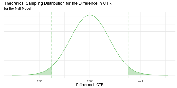
The null model tell us that the mean difference in CTR between the two versions is zero, that if we were able to repeat the experiment over and over again with 1000 visitors in each group and measure the difference in CTR, it would follow the shown Normal distribution.

The shaded green area represents 5% of the area under the curve, 2.5% each side. Since the difference in CTR is negative when Version B performs worse, we have to take both sides into account. So, if \(H_0\) is true, upon measuring the difference in CTR, there is a 5% chance that it falls in the shaded area and we incorrectly reject \(H_0\), committing a type I error or a false positive (we thought we detected an effect that wasn’t really there).

The Alternative Model and the Quest for Power

We are performing a two-sided hypothesis test since we want to detect if version B is doing better OR worse. The alternative hypothesis would therefore be that “there is some difference between the click-through rates of versions A and B,” i.e. \(CTR_a \ne CTR_b\).

Now suppose the alternative hypothesis \((H_A)\) is true and the CTR for Version B is indeed 1%? In this case, we’d expect most of our difference-between-proportions calculations \((CTR_b - CTR_a)\) to be closer to 0.005 (0.010 - 0.005) than to 0. Referencing the null model, when this value is greater than the critical value, we reject \(H_0\). This is exactly what we want. If \(H_A\) is true, we hope to gather enough evidence to reject \(H_0\). This then begs the question, “How likely are we to incorrectly fail to reject \(H_0\)?” When \(H_A\) is true and we fail to reject \(H_0\), we commit a type II error or a false negative (we thought we didn’t detect an effect, though there really was one). It’s important to understand type I and II errors in order to understand power. To summarize,

When \(H_0\) is true,
- we hope that enough data will show us a net zero effect and lead us to fail to reject \(H_0\).
- if we reject \(H_0\), we’ve committed a type I error (false positive).
When \(H_A\) is true,
- we hope to gather enough evidence to lead us to reject \(H_0\) and conclude that we’ve detected an effect.
- if we fail to reject \(H_0\), we’ve committed a type II error (false negative).

The alternative model is centred at the effect size. If there is indeed an effect of a certain size, we expect most measurements to be close to that size. The standard error is not exactly the same as the null model. If we believe the alternative model to be true, then we believe that the CTR for each version is different so we don’t use a pooled SE.

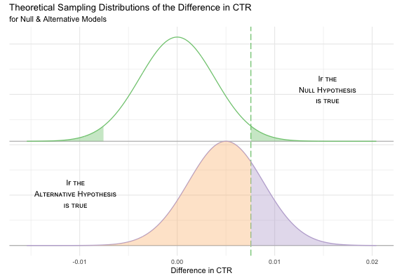
Notice how the critical value that we use for deciding whether to reject (or fail to reject) \(H_0\) divides the alternative model into two sections. Remember, we don’t know if \(H_A\) is true or not. Our experiments are based on \(H_0\) and we’re trying to decide whether to reject it or not, so the critical value doesn’t change when we introduce the alternative model. So what do these two areas in the alternative model represent?

Well, if the alternative hypothesis is true, we’d only believe it after rejecting \(H_0\), so we’d need to measure a difference in CTR that is greater than the critical value. That’s the purple shaded area, so we’d only have about a 25% probability of detecting an effect. This is a measure of the statistical power of our experiment. It is the probability of rejecting \(H_0\), given that \(H_A\) is true. In our experiment, we don’t know if \(H_A\) is true but if it is, we have a 25% chance of detecting an effect size of \(\frac{1}{2}\%\).

If our measurement is less than the critical value, we’d commit a type II error. That’s the orange shaded area, so we’d have a 75% probability of a false negative. This measurement is called “beta” \((\beta)\).

\(\alpha\) is the probability of committing a type I error when \(H_0\) is true.

\(\beta\) is the probability of committing a type II error when \(H_A\) is true.

power is the probability of detecting an effect when \(H_A\) is true.

It’s easy to calculate the power. Previously, we calculated the critical value based on the null model and \(\alpha\). Now, we use that critical value with the alternative model to calculate power. Note that this time, we’ll use the non-pooled standard error for the difference between proportions since we’re considering the alternative model.

# Previously, we calculated critical value based on null model
> critical_value <- qnorm(alpha / 2, sd = SE_pooled, lower.tail = FALSE)

# Calculate SE for difference between proportions based on alternative model
> SE <- sqrt((p_a * q_a / n) + (p_b * q_b / n))

# Now use critical value and SE to calculate power based on alternative model
> delta_CTR <- 0.005 # the size of the effect we want to detect
> power <- pnorm(critical_value,
+                mean = delta_CTR,
+                sd = SE,
+                lower.tail = FALSE)
>
> c(SE, power)
[1] 0.003856812 0.253223604

Sample Size and Increasing Power

It’s easy to see that the more you shift the alternative model to the right (see Figure 2), the larger the purple shaded area, and therefore the higher the probability of rejecting \(H_0\). What this tells us is that it’s easier to detect larger effect sizes. So by simply increasing the effect size, we can increase the power. However, this is not always a practical solution. In our case, we’re interested in detecting a specific increase in CTR so detecting a larger increase is not very helpful.

Another way to increase power, that may not be as obvious, is to alter the distributions so that they aren’t as wide. This results in a lower critical value, so we’re moving the dividing line to the left (instead of shifting the alternative model to the right), resulting in lower \(\beta\) and larger power. To narrow the distribution, we need a smaller standard error. We can decrease the standard error by increasing our sample size. Let’s double the sample size and redo all our calculations.

> n <- 2000
>
> SE_pooled <- sqrt(1/n) * sqrt((p_a + p_b) * (1 - (p_a + p_b) / 2))
> critical_value <- qnorm(alpha / 2, sd = SE_pooled, lower.tail = FALSE)
>
> SE <- sqrt((p_a * q_a / n) + (p_b * q_b / n))
> power <- pnorm(critical_value,
+                mean = delta_CTR,
+                sd = SE,
+                lower.tail = FALSE)
>
> c(SE_pooled, SE, critical_value, power)
[1] 0.002728324 0.002727178 0.005347416 0.449315734

Let’s compare the values before and after.

n	SE (pooled)	SE (non-pooled)	Critical Value	Power
1000	0.003858432	0.003856812	0.007562388	0.253223604
2000	0.002728324	0.002727178	0.005347416	0.449315734

Doubling the sample size resulted in smaller standard errors, lowering the critical value and increasing the power. We now have a 45% chance of detecting an effect at the cost of waiting for more people to visit the website. But 45% is still not that good. What if we wanted to power our experiment to have an 90% chance at detecting an effect? How many visitors would we need?

Sample Size for Difference Between Proportions

Let’s calculate the critical value in terms of n using the null and alternative models. Since we are referring to the same critical value in each case, we can then equate our two formulae for this value and solve for n.

From our null model, we already know that we can calculate the critical value for some given standard error SE with qnorm.

qnorm(alpha / 2, mean = 0, sd = SE_pooled, lower.tail = FALSE)

However, we don’t know SE_pooled yet since we need to know n to calculate it. We therefore need to separate the SE term out of the qnorm function. If we don’t include distribution parameters, then qnorm assumes a standard normal distribution. To convert back to our distribution, we multiply by SE. Let’s also replace qnorm(x, lower.tail = FALSE) with the more compact form qnorm(1 - x) or -qnorm(x). This gives us:

-qnorm(alpha / 2) * SE_pooled

Now, let’s calculate the same critical value using the alternative model. This model is shifted by the effect size (p_b - p_a), so we’ll need to take this into account too. This gives us:

(p_b - p_a) + qnorm(beta) * SE

or, since power = 1 - beta and qnorm(1 - x) = -qnorm(x),

(p_b - p_a) - qnorm(power) * SE

Now let’s equate and solve for n. Using \(\Phi\) to represent the standard normal cumulative distribution function pnorm(x), and therefore \(\Phi^{-1}\) for qnorm(x),

\[-\Phi^{-1}_{\alpha/2} \space SE_{pooled} = (\hat{p}_b - \hat{p}_a) - \Phi^{-1}_{power} \space SE\]

\[\hat{p}_b - \hat{p}_a = \Phi^{-1}_{power} \space SE - \Phi^{-1}_{\alpha/2} \space SE_{pooled}\]

Recall,

\[SE = \sqrt{\dfrac{\hat{p}_a \hat{q}_a + \hat{p}_b \hat{q}_b}{n}} = \sqrt\frac{1}{n} \space \sqrt{\hat{p}_a \hat{q}_a + \hat{p}_b \hat{q}_b} = \sqrt\frac{1}{n} \space X, \] \[\text{ where } X = \sqrt{\hat{p}_a \hat{q}_a + \hat{p}_b \hat{q}_b}\]

and,

\[SE_{pooled}= \sqrt{\frac{1}{n}} \space \sqrt{(\hat{p}_a+\hat{p}_b)\left(1-\frac{\hat{p}_a+\hat{p}_b}{2}\right)} = \sqrt\frac{1}{n} \space Y,\]

\[\text{ where } Y = \sqrt{(\hat{p}_a+\hat{p}_b)\left(1-\frac{\hat{p}_a+\hat{p}_b}{2}\right)}\]

Substituting,

\[\hat{p}_b - \hat{p}_a = \Phi^{-1}_{power} \space \sqrt\frac{1}{n}\space X - \Phi^{-1}_{\alpha/2} \space \sqrt\frac{1}{n}\space Y\]

\[\sqrt{n}\space(\hat{p}_b - \hat{p}_a) = \Phi^{-1}_{power} \space X - \Phi^{-1}_{\alpha/2}\space Y\]

\[n = \left(\frac{\Phi^{-1}_{power} \space X - \Phi^{-1}_{\alpha/2}\space Y}{\hat{p}_b - \hat{p}_a}\right)^2\]

\[n = \left(\frac{\Phi^{-1}_{power} \sqrt{\hat{p}_a \hat{q}_a + \hat{p}_b \hat{q}_b} - \Phi^{-1}_{\alpha/2}\space \sqrt{(\hat{p}_a+\hat{p}_b)\left(1-\frac{\hat{p}_a+\hat{p}_b}{2}\right)}}{\hat{p}_b - \hat{p}_a}\right)^2\]

Sample Size for Difference Between Means

Similarly, if you are testing the difference between means, you can derive a similar formula to calculate the sample size by using the formula for the standard error of the difference between means. Because the pooled and non-pooled estimates tend to be so similar and the math tends to get out of hand, particularly in the case of difference between means, you’re likely to see the formula derived without using a pooled SE. \[n=\dfrac{2 s_a s_b\left(\Phi^{-1}_{power} - \Phi^{-1}_{\alpha/2} \right)^2}{(\hat{\mu}_b - \hat{\mu}_a)^2}\] where

\(s_a, s_b =\) sample standard deviations

\(\hat{\mu}_a, \hat{\mu}_b=\) sample means

In R,

calculate_sample_size <- function(ctr_a, ctr_b, power, alpha = 0.05) {
  p_a <- ctr_a
  p_b <- ctr_b

  n <- ((qnorm(power)*sqrt((p_a*q_a)+(p_b*q_b))
        -qnorm(alpha/2)*sqrt((p_a+p_b)*(1-(p_a+p_b)/2)))/ (p_b-p_a))^2

  ceiling(n)
}

Let’s test it using the two power values we calculated earlier.

> calculate_sample_size(ctr_a = 0.005, ctr_b = 0.010, power = 0.2532)
[1] 1000

> calculate_sample_size(ctr_a = 0.005, ctr_b = 0.010, power = 0.4493)
[1] 2000

We can now answer the question of how many visitors we would need to power our experiment to have a 90% probability of detecting an effect size of \(\frac{1}{2}\%\).

> calculate_sample_size(ctr_a = 0.005, ctr_b = 0.010, power = 0.90)
[1] 6256

So we’d need 6,256 visitors for each version of our banner image, or a total of 12,512 visitors.

Using R’s Built-in Functions

Ok, that was a lot of math! Admittedly, you’ll never need to write your own functions to determine sample size or power. R has some built-in functions just for this (in the stats package).

Let’s check our results with power.prop.test. This function accepts several arguments related to calculating power and calculates the NULL argument (the one you leave out).

> power.prop.test(p1 = 0.005, p2 = 0.010, power = 0.90)

     Two-sample comparison of proportions power calculation

              n = 6255.093
             p1 = 0.005
             p2 = 0.01
      sig.level = 0.05
          power = 0.9
    alternative = two.sided

NOTE: n is number in *each* group

If we round n up, we get the same result that we’d need 6256 visitors for each group/version. If you’re comparing means, use power.t.test.

The power.prop.test function does pretty much the same math that’s been discussed so far but it can handle both one and two-sided tests. It uses a formula to calculate power. To solve for other variables, such as sample size, it uses stats::uniroot to solve for the missing argument of the power formula.

A Peek under the Hood

All the math we’ve done so far leads to the expression used in power.prop.test to calculate power. As we’ve seen before,

critical_value <- qnorm(alpha / 2, sd = SE_pooled, lower.tail = FALSE)

and

power <- pnorm(critical_value,
               mean = delta_CTR,
               sd = SE_pooled,
               lower.tail = FALSE)

These can be re-written as

\[Z^*=-\Phi^{-1}_{\alpha/2}\space SE_{pooled}\]

and

\[\begin{aligned} \text{Power} &= 1-\Phi\left(\frac{Z^*-(\hat{p}_b-\hat{p}_a)}{SE}\right) \\ &= \Phi\left(\frac{\hat{p}_b-\hat{p}_a-Z^*}{SE}\right) \end{aligned}\]

Substituting \(Z^*\) in the power equation and both \(SE\), and \(SE_{pooled}\) as previously defined,

\[\text{Power}=\Phi\left(\frac{\hat{p}_b-\hat{p}_a+\Phi^{-1}_{\alpha/2} \sqrt\frac{1}{n} \sqrt{(\hat{p}_a+\hat{p}_b)\left(1-\frac{\hat{p}_a+\hat{p}_b}{2}\right)}}{\sqrt\frac{1}{n}\space\sqrt{\hat{p}_a (1-\hat{p}_a) + \hat{p}_b (1-\hat{p}_b)}}\right)\]

\[=\Phi\left(\frac{\sqrt{n}\space(\hat{p}_b-\hat{p}_a)+\Phi^{-1}_{\alpha/2} \sqrt{(\hat{p}_a+\hat{p}_b)\left(1-\frac{\hat{p}_a+\hat{p}_b}{2}\right)}}{\sqrt{\hat{p}_a (1-\hat{p}_a) + \hat{p}_b (1-\hat{p}_b)}}\right)\]

Now, if you take a look at the power.prop.test function code, you can see this expression being used for calculating power.

> power.prop.test
function (n = NULL, p1 = NULL, p2 = NULL, sig.level = 0.05, power = NULL,
    alternative = c("two.sided", "one.sided"), strict = FALSE,
    tol = .Machine$double.eps^0.25)
{
  .
  .
  .
    p.body <- if (strict && tside == 2)
        quote({
          .
          .
          .
        })
    else quote(pnorm((sqrt(n) * abs(p1 - p2) - (qnorm(sig.level/tside,
        lower.tail = FALSE) * sqrt((p1 + p2) * (1 - (p1 + p2)/2))))/sqrt(p1 *
        (1 - p1) + p2 * (1 - p2))))
    if (is.null(power))
        power <- eval(p.body)
  .
  .
  .
}

This is only meant to give you an understanding and appreciation of power.prop.test. There’s a lot of math packed in there but ultimately, you only need to understand how to use it, not so much how it works.

Early Peeking

Image by Lili Vieira de Carvalho

Waiting for 12,512 visitors to your website may not be feasible unless you run a high-traffic site like Amazon or Facebook. Suppose you’re only getting, say, about 100 visitors per day. At that rate, you’d need to wait 125 days or about 4 months. Short of increasing traffic to the site, is there anything else we can do?

Well, if there’s a strong enough signal, we could see our desired \(\frac{1}{2}\%\) increase in CTR sooner than expected. What if we continuously monitored the results by checking the CTR of each version at the end of each day to see where we’re at? Colloquially, this is known as “peeking.”² What if after the first day of the experiment, we saw a difference of over 0.005 (our target CTR increase)? Would you believe it? What if it were over 0.005 after 1 month? Do we need to wait for 4 months before believing in a noted difference in CTR of over 0.005?

We know that if we wait for all 12,512 visitors, there’s a 90% chance of detecting the effect; the power of the experiment. So if we have just one shot at measuring the difference in CTR between versions A and B after waiting 4 months, we’re “90% confident” of the result. But how confident are we when we peek at the results on a daily or weekly basis? There is definitely a difference between a 0.005 difference in CTR in one day, or even 10, than a similar difference over a 4 month period, so how can we account for this difference?

What’s Wrong with Peeking at the Results?

Verifying Type I and II Error Rates

To understand what can go wrong with early peeking, let’s first verify the error rates involved with our experiment. Recall that we’ve chosen \(\alpha=0.05\) and \(\beta=0.10\) \((\beta=1-power=1-0.90)\) for our experiment.

This means

if \(H_0\) is true, there’s a 5% chance of a false positive
if \(H_A\) is true, there’s a 10% chance of a false negative

Let’s simulate this in R to verify these error rates. The code below is also available as a gist.

Simulation Code

#' Simulate visitors clicking on banner image version A and B
#'
#' @param p_a Known CTR for Version A
#' @param p_b Target CTR for Version B
#' @param impressions The total number of impressions
#'
create_sim_data <- function(p_a, p_b, impressions) {
  p_delta <- abs(p_a - p_b)
  tibble(version = sample(0:1, size = impressions, replace = TRUE),
         response = rbinom(version, size = 1, prob = p_a + version * p_delta)) %>%
    mutate(version = ifelse (version, "B", "A"),
           response = ifelse (response, "click", "no_click"))
}

#' Calculate Standard Deviation based on Wald Test.
#'
#' Z-statistic is difference in log odds ratio divided by
#' the std. dev. of the sampling distribution of the diff in log odds.
#'
#' @param sim_data Simulation data
#' @param n First n visits to use
#' @return Z-statistic
#'
calc_z_statistic_wald <- function(sim_data, n) {
  counts <- table(sim_data[1:n,])
  l <- log(counts)
  se <- sqrt(sum(1 / counts))
  abs(((l[2, 1] - l[2, 2]) - (l[1, 1] - l[1, 2])) / se)
}

#' Calculate Standard Deviation based on a logistic regression model
#' using `glm`. We can get the z-statistic from the `summary` function.
#'
calc_z_statistic_logit <- function(counts, n) {
  # counts <- table(sim_data[1:n,])
  versions <- c("A", "B")
  glm(counts ~ versions, family = binomial) %>%
    summary %>%
    (function(s) s$coefficients[2, "z value"])
}

#' Minimum number of visitors in order to form
#' a 2x2 contingency table with all non-zero counts
#' so that we can get some meaningful statistics
#'
#' @param sim_data tibble of "version" (A, B) and "response" (click, no-click)
#' @return number representing minimum number of visitors
#'
find_min_n <- function(sim_data) {
  for (n in 1:nrow(sim_data)) {
    counts <- table(sim_data[1:n,])
    if (all(dim(counts) == c(2, 2)) && min(counts) > 0) {
      return(n)
    }
  }
  n
}

#' Simulation of visitors to website
#'
#' For each impression, either Version A or Version B is served.
#' The probability of the visitor clicking through depends on
#' specified arguments.
#'
#' @param p_a Known CTR for Version A
#' @param p_b Target CTR for Version B
#' @param impressions The total number of impressions
#' @param zfn Function to calculate Z-statistic
#' @param alpha Type I error rate
#' @param num_checks Number of checks, evenly spaced. If `num_checks == 1`,
#'        the check is done after all impressions. If `num_checks > 1`,
#'        you are peeking early and `alpha` should be adjusted accordingly.
#'
#' @return TRUE if null hypothesis is rejected, else FALSE
#'
simulate <- function(p_a, p_b, impressions, zfn, alpha, num_checks=1) {
  critical_value <- -qnorm(alpha / 2)
  sim_data <- create_sim_data(p_a, p_b, impressions)
  min_n <-  find_min_n(sim_data)

  stops <- ceiling(seq(from = 1,
                       to = impressions,
                       length.out = (num_checks+1))[-1])

  for (n in stops) {
    z <- abs(zfn(sim_data, max(min_n, n)))
    if (z > critical_value) return (TRUE)
  }
  FALSE
}

First, the parameters for our experiment.

> p_a <- 0.005
> p_b <- 0.010
> impressions <- 2 * 6256
> alpha <- 0.05
> repetitions <- 5000

Using the create_sim_data function above, we’ll simulate visitors to the website. Each visitor is randomly assigned version A or B and whether or not it resulted in a click through. We can use the table function in R to create a contingency table of the results.

> sim_data <- create_sim_data(p_a, p_b, impressions)
> table(sim_data)
       response
version click no_click
      A    41     6207
      B    64     6200

The Z-statistic can then be calculated. The included code shows two ways to do this. calc_z_statistic_wald is based on the Wald test (for details on this, see the StatQuest video, Log of Odds Ratio). calc_z_statistic_logit uses logistic regression to determine if the increment of the log odds from A to B is significant.

> calc_z_statistic_wald(sim_dta, impressions)
[1] 2.222835

> calc_z_statistic_logit(sim_dta, impressions)
[1] 2.222835

We can then compare the Z-statistic to the critical value based on \(\alpha\) and decide if to reject \(H_0\) or not. We’ll repeat this experiment 5000 times. Since we know there is a difference in CTR, we expect to have a type II error rate of approximately 10% (or power of approximately 90%).

The simulate function simulates impression number of users visiting a website. Each visitor is randomly assigned version A or version B. The probability of a click-through by the visitor is simulated with the probabilities (p_a and p_b).

By default, it will only perform the hypothesis test based on all the results. To simulate checking the results at fixed, periodic intervals, supply the optional num_checks argument.

> 1:repetitions %>%
+   map_lgl(~simulate(p_a,
+                     p_b,
+                     impressions,
+                     calc_z_statistic_wald,
+                     alpha)) %>%
+   mean()
[1] 0.9114

After 5000 experiments, 91% of them resulted in detecting an effect, so we incorrectly failed to reject \(H_0\) 9% of the time, pretty much what we expected.

What if there were no difference to detect? In this case, we’d expect a type I error rate of approximately 5%.

> 1:repetitions %>%
+   map_lgl(~simulate(p_a,
+                     p_a, # no difference in CTR
+                     impressions,
+                     calc_z_statistic_wald,
+                     alpha)) %>%
+   mean()
[1] 0.0486

So we incorrectly rejected \(H_0\) 5% of the time, which is what we expected.

Type I and II Error Rates when Continuously Monitoring

We’ve just seen that if we have the luxury of waiting for the required number of visitors needed to properly power our experiment, that the error rates are pretty much spot on. Now let’s stop our experiment as soon as we get promising results and see what happens. We’ll do this by setting num_checks = impressions to check the results after every visit.

Ironically, simulating early stopping takes longer than the previous simulations, so let’s add a progress bar.

> pb <- txtProgressBar(min = 1, max = repetitions, style = 3)
>
> power <- 1:repetitions %>%
+   map_lgl(function(n) {
+     setTxtProgressBar(pb, n)
+     simulate(p_a,
+              p_b,
+              impressions,
+              calc_z_statistic_wald,
+              alpha,
+              num_checks = impressions)
+   }) %>%
+   mean()
|==========================================================================| 100%
> power
[1] 0.9502

The type II error rate is 5%. This may seem like an improvement but by prematurely stopping as soon as we think we have significant results, we end up being over-confident that we’ve detected an effect. Not too devastating if, in fact, there was an effect. But, what happens when \(H_0\) is true?

I’ll leave out the progress bar code for simplicity.

> 1:repetitions %>%
+   map_lgl(~simulate(p_a,
+                     p_a, # no difference in CTR
+                     impressions,
+                     calc_z_statistic_wald,
+                     alpha,
+                     num_checks = impressions)) %>%
+   mean()
[1] 0.2146

Early stopping resulted in a false positive rate of 21%. That’s about a 400% increase in the false positive rate! This means that when there is no difference in CTR, there’s a much stronger possibility that we’ll incorrectly think there is.

The Bonferroni Correction

We’ve just seen that early stopping leads to higher overall error rates. Why is this?

Let \(R_i\) = “\(H_0\) is rejected for test \(i\) of \(m\).” Then, if we perform two tests, by the law of probabilities,

\[\begin{aligned} P(R_1 \cup R_2) &= P(R_1) + P(R_2) - P(R_1 \cap R_2) \\ &\le P(R_1) + P(R_2) \end{aligned}\]

We only care about the probability of at least one of the events happening since we stop early (as soon as \(H_0\) of a test gets rejected), thus \(P(R_1 \cup R_2) \). Extending this to \(m\) tests,

\[\begin{aligned} P(R_1 \cup R_2 \cup ... \cup R_m) &= P(R_1) + P(R_2) + ... + P(R_m) - P(R_1 \cap R_2 \cap ... \cap R_m) \\ &\le P(R_1) + P(R_2) + ... + P(R_m) \end{aligned}\]

Since \(P(R_i) = \alpha\), for all \(i\) in \(1…m\),

\[\begin{aligned} P(R_1 \cup R_2 \cup ... \cup R_m) &\le P(R_1) + P(R_2) + ... + P(R_m) \\ &\le m\alpha \end{aligned}\]

Therefore, to limit the family-wise error rate (FWER) to a maximum of \(\alpha\), we need to use a significance level of \(\alpha/m\) for each test. So, replacing \(\alpha\) with \(\frac{\alpha}{m}\),

\[\text{FWER }\le m \left(\frac{\alpha}{m}\right)=\alpha\]

Let’s verify that FWER < \(\alpha\) when \(H_0\) is true. We’ll peek 10 times per experiment.

> m <- 10
>
> FWER <- 1:repetitions %>%
+   map_lgl(~simulate(p_a,
+                     p_a,
+                     impressions,
+                     calc_z_statistic_wald,
+                     alpha/m, # notice the change in the significance level
+                     num_checks = m)) %>%
+   mean()
>
> FWER
[1] 0.0096

So we’re able to keep the FWER below \(\alpha\) when \(H_0\) is true. On the other hand, if you simulate \(H_A\) being true, you’ll notice a drop in power. This makes sense. Referring again to the null/alternative models, if you keep everything else constant and only shift the critical value to the right, you decrease power. Let’s see what power.prop.test gives us. Remember that n is the number of visitors per group (impressions/2).

> power.prop.test(n = impressions/2,
+                 p1 = p_a,
+                 p2 = p_b,
+                 sig.level = alpha/m)$power
[1] 0.6679868

So the power has decreased and consequently, the type II error rate has increased. This reduction in power is OK if we end up stopping early. The key point here is that if we peek early and reject \(H_0\text{,}\) we’ve convinced ourselves that (with the correction) there was enough evidence to do so, otherwise we continue the experiment.

It should be noted that the FWER is considered quite conservative and in practice, you’ll likely see False Discovery Rate (FDR) used in place of type I error rates. See False Positives, FWER, and FDR Explained for an explanation of the difference between FWER and FDR.

Practical Methods for Early Stopping

We’ve seen that we can peek early if we do a Bonferroni correction. However, this requires that we decide beforehand on the number of times we’re going to peek, so while useful as a correction for multiple testing, it may not always be practical in real-world A/B testing. There are several strategies used in practice for continuous monitoring of A/B experiments. They are beyond the scope of this article but I’ll briefly mention some of them here.

Sequential Hypothesis Testing, a broad term used to refer to a family of testing frameworks, attempts to overcome the problem of using pre-determined sample sizes. P-value thresholds are dynamically determined based on the available data at the time of peeking. This dynamic threshold adjusting takes us out of the realm of (frequentist) fixed-horizon hypothesis testing.

Multi-Armed Bandits is a variation to sequential testing that incorporates early stopping with the ability to optimize over multiple testing variations. For example, we could test 5 different new versions, quickly dropping poorly performing versions while continuing to test those that are performing better, allowing a business to reach decisions more quickly.

There’s also the Bayesian approach to A/B testing which can incorporate prior knowledge, say, from past experiments. Additionally, unlike the frequentist approach, you can also answer questions like “What is the probability that version B is better than version A?”.⁹