An Introduction to Machine Learning Optimization

In many supervised machine learning algorithms, we are trying to describe some set of data mathematically. In order to do this, we need to determine the coefficients of the formula we are trying to model. In machine learning, this is done by numerical optimization.

For example, if we are trying to fit the equation $y = ax^2 + bx + c$ to some dataset of $(x, y)$ value-pairs, we need to find the values of $a$, $b$ and $c$ such that the equation best describes the data. This article will use the Gradient Descent optimization algorithm to explain the optimization process. While it is not used in practice in its pure and simple form, it is a good pedagogical tool for illustrating the basic concepts of numerical optimization. Towards the end, I’ll briefly describe the optimization methods you can expect to find practice.

Code examples are in R and use some functionality from the tidyverse and plotly packages.

A Toy Dataset

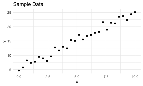
Two dimensional data is good for illustrating optimization concepts so let’s starts with data with one feature paired with a response. The data might represent the distance an object has travelled (y) after some time (x), as an example. However, I’ll use a very simple, meaningless dataset so we can focus on the optimization.

Here, I generate data according to the formula $y = 2x + 5$ with some added noise to simulate measuring data in the real world. The data points follow a linear pattern so we will try to fit $y = mx + c$ to the data and estimate values for coefficients $m$ and $c$. We expect to get something close to $m=2$ and $c=5$. In machine learning, we usually refer to the coefficients as parameters and symbolize them with the Greek letter $\theta$ so let’s rewrite the formula as $y = \theta_0 + \theta_1x$.

# Number of examples (number of data points)
n <- 30

# These are the true parameters we are trying to estimate
true_theta0 <- 5
true_theta1 <- 2

# This is the function to generate the data
f <- function(x, theta0, theta1) theta0 + theta1*x

# Generate some x values
x <- seq(0, 10, len=n)

# Generate the corresponding y values with some noise
set.seed(4836)
y <- sapply(x, f, true_theta0, true_theta1) + rnorm(n)

This is a two-dimensional plot of the data. It looks linear so it’s reasonable to model the data with a straight line.

Graph of sample linear data

First, let’s skip ahead and fit a linear model using R’s lm to see what the estimates are. These are the best estimates for these data using the ordinary least squares (OLS) method. It is typical to use OLS for linear models since it is the best linear unbiased estimator (BLUE) so that’s what I’ll use for our upcoming home-grown optimizer.

(lm_thetas <- lm(y ~ x)$coefficients)

output:

(Intercept)           x
   5.218865    1.985435

The estimates are $\theta_0 = 5.218865$ and $\theta_1 = 1.985435$, which are close to the true values of 5 and 2. Now, let’s calculate these values for ourselves.

Minimizing the Residual Sum of Squares

OLS uses the residual sum of squares (RSS) as a measure of how well our model fits the data. The lower the value the better, hence we will be minimizing the RSS in determining suitable values for $\theta_0$ and $\theta_1$.

\[RSS = \sum (y - \hat{y})^2\]

where $y$ represents the actual values from our data (the observed values) and $\hat{y}$ represents the predicted values of $y$ based on the estimated parameters. And in code,

rss <- function(theta0, theta1) {
  residuals <-  y - f(x, theta0, theta1)
  sum(residuals^2)
}

In order to gain intuition into why we want to minimize the RSS, let’s vary the values of one of the parameters while keeping the other one constant. We’ll focus on values of $\theta_0$ just below and above the true value of $5$ while keeping the value of $\theta_1$ fixed at the estimated value (according to lm). This will allow us to easily see what the estimated value of $\theta_0$ should be, approximately. We can do this for $\theta_1$ as well.

Code to generate RSS 2D graphs

theta_seq <- function(theta, delta, length)
  seq(theta - delta, theta + delta, length=length)

theta0s <- theta_seq(true_theta0, delta=1, length=200)
RSS0 <- sapply(theta0s, rss, theta1=lm_thetas[2])

p1 <- ggplot() + geom_line(aes(theta0s, RSS0)) +
  labs(title = "Residual Sum of Squares",
       subtitle = expression(Varying~theta[0]),
       x = expression(theta[0]), y = "RSS")

theta1s <- theta_seq(true_theta1, delta=1, length=200)
RSS1 <- sapply(theta1s, rss, theta0=lm_thetas[1])

p2 <- ggplot() + geom_line(aes(theta1s, RSS1)) +
  labs(title = "Residual Sum of Squares",
       subtitle = expression(Varying~theta[1]),
       x = expression(theta[1]), y = "RSS")

gridExtra::grid.arrange(p1, p2, ncol=2)

Attribution: Code folding blocks from endtoend.ai’s blog post, Collapsible Code Blocks in GitHub Pages.

RSS graphs showing minimum

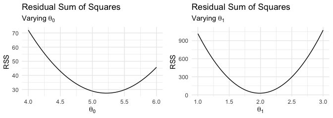
You can immediately see that a value of approximately $5.2$ for $\theta_0$ will give the minimum RSS value. Likewise, a value of approximately $2$ for $\theta_1$ achieves the minimum RSS value.

NOTE: There is only one minimum RSS value that we want to achieve while varying both parameters simultaneously. The two-dimensional graphs only illustrate one parameter being varied at a time and are for illustration purposes only.

RSS in 3D

Since we are varying two parameters simultaneously in our quest for the best estimates that minimize the RSS, we are searching a 2D parameter space. To see how the RSS varies with both parameters, we can show this as a 3D plot.

Code to generate RSS 3D plot

# Construct x and y grid elements
delta <-  2
theta0s_3d <- theta_seq(true_theta0, delta, length=200) # real value = 5
theta1s_3d <- theta_seq(true_theta1, delta, length=200) # real value = 2

# Construct z grid by computing predictions for all x/y pairs
cross <-  tidyr::crossing(theta0s_3d, theta1s_3d)
z_grid <- apply(cross, 1, function(x) rss(x[1], x[2]))
z_grid <- matrix(z_grid, nrow = length(theta0s)) #reshape z

# Plot using plotly
plot_ly(showscale=F) %>%
  layout(scene = list(xaxis = list(title = 'theta_0'),
                      yaxis = list(title = 'theta_1'),
                      zaxis = list(title = 'RSS'))) %>%

  add_surface(x = ~theta0s_3d, y = ~theta1s_3d, z = ~z_grid,
              colorscale = list(list(0, "#DDD"), list(1, "blue")))

Attribution: Original Plotly code for showing RSS of 2D parameter space in 3D was taken from a lecture in my Master of Data Science program at the University of British Columbia.

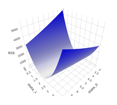
RSS graph with both parameters varying

You can see that as $\theta_1$ moves towards its optimal value, the RSS drops quickly but that the descent is not as rapid as $\theta_0$ moves towards its optimal value. We’ll see this again when I cover Gradient Descent shortly.

Where is the minimum RSS value?

A grid of RSS values was created to match the a discrete version of the 2D parameter space for the purposes of plotting. We can find where in this grid lies the minimum RSS value.

which(z_grid == min(z_grid), arr.ind = TRUE)

output:

     row col
[1,] 100 110

Taking a peek into the grid,

RSS grid table results

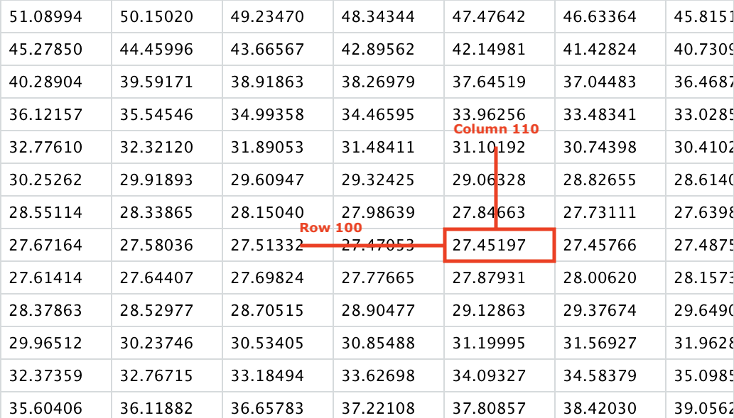
As mentioned earlier, you can see that along the $\theta_0$ axis (looking across the row values), the rate of change in value is lower than along the $\theta_1$ axis (looking up and down the row values), which explains the shape of the surface in the 3D plot.

Caution: As the grid is not continuous, this is not necessarily the absolutely lowest possible RSS for the given data. It’s just the lowest value that we’ve computed for all the combinations of $\theta_0$ and $\theta_1$ that were chosen for the discrete grid. But this minimum value should be close to the actual minimum.

The Cost Function

While the RSS measures the model’s goodness of fit, it can grow really large, especially as the number of data examples (sample size) increases. To measure the “cost” of a particular combination of parameters, let’s look the the mean squared error (MSE) instead. For our dataset of $n$ examples, the MSE is simply $\frac{RSS}{n}$.

\[MSE = \frac{1}{n} \sum\limits_{i=1}^n (y_i - \hat{y_i})^2\]

where $\hat{y_i}$ is the predicted or hypothesized value of $y_i$ based on the parameters we choose for $\theta$.

The cost function is also known as the loss function but I prefer the term cost because intuitively, it’s telling us how expensive it is to use a specific combination of parameters. We seek to lower this cost through optimization. I will use some of the same terminology that Chris McCormick uses in his blog post on Gradient Descent Derivation in case you want to cross reference this post for some of the derivation details that I won’t go into.

It should be noted that both RSS and MSE can be used as a cost function with the same results as one is just a multiple of the other. In fact, since we can multiply by any number, you’ll typically see $\frac{1}{2n}$ instead of $\frac{1}{n}$ as it makes the ensuing calculus a bit easier.

Substituting $h_{\theta}(x)$ (hypothesis function) for $\hat{y}$ and multiplying by $\frac{1}{2}$ to simplify the math to come, we can write the loss function as

\[J(\theta) = \frac{1}{2n} \sum\limits_{i=1}^n (y_i - h_{\theta}(x_i))^2\]

The $\theta$ subscript in $h_{\theta}$ is to remind you that $h$ is a function of $\theta$ which is important when taking the partial derivative, which we’ll see shortly. As a reminder, we’re trying to solve the following function.

\[h_{\theta}(x) = \theta_0 + \theta_1x\]

NOTE: The cost function varies depending on the objective of your model. In this example, we’re trying to fit a line to a set of points. On the other hand, if we were trying to classify data (binary or multinomial logistic regression), we’d use a different cost function.

Gradient Descent

To recap, we’re trying to solve the function $h_{\theta}$ for $\theta_0$ and $\theta_1$. Based on values we select for them, we can calculate the cost using the cost function $J(\theta)$. We want to minimize this cost. Let’s say we pick random values for $\theta_0$ and $\theta_1$. This puts us somewhere in the parameter space with some cost value. We do not know if this is the best location that gives the lowest cost. So, after we calculate this cost, how do we adjust $\theta_0$ and $\theta_1$ such that the cost goes down?

Gradient ascent and descent

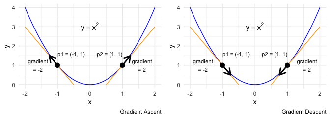
Let’s look at a simple example that only involves $x$ and $y$. If $y = x^2$ then the gradient at any point $x$ is defined by $\frac{dy}{dx} = 2x$. Consider the points $p1$ and $p2$. At $p1$ the gradient is $-2$ (negative) while at $p2$ the gradient is $2$ (positive). If I follow the sign of the gradient, decreasing $x$ when the gradient is negative and increasing $x$ when the gradient is positive, then I’ll be moving away from the minimum. So, just getting the gradient at a specific point tells me the direction of ascent. This is Gradient Ascent. What we want, however, is to move in the opposite direction.

To move the point $p2$ towards the minimum, we need to decrease $x$. In reality, we won’t know what value of $x$ achieves the minimum, only that moving in the opposite direction of the gradient can move us towards the minimum. In this example, if we move by the full value of the gradient, we’d overshoot the minimum and start to ascend on the other side. What we need to do is subtract a fraction of the gradient. This fraction is called the learning rate. With a learning rate $\alpha$, we’d adjust $x$ as follows.

\[x_{new} = x_{old} - \alpha\frac{dy}{dx} \biggr\rvert_{x=x_{old}}\]

For example, with a learning rate $\alpha=0.1$,

\[x_{new} = 1 - 0.1 (2) = 0.8\]

We’ve just used gradient descent to move a bit closer to the minimum. At this point, our gradient has changed. It’s now $\frac{dy}{dx}\rvert_{x=0.8} = 1.6$. Notice that as we move closer to the minimum, the gradient decreases which means that we move in smaller increments as we approach the minimum which is precisely what we want. That is, the further away we are from the minimum, the faster we descend towards it; the closer we get, the slower we approach.

Partial Derivatives

The above example involved adjusting one parameter, $x$. If we go back to our original toy dataset, our $x$ and $y$ values are fixed by our data. What we want to adjust are the parameters $\theta_0$ and $\theta_1$. We have one derivative but need to adjust multiple (two in our case) parameters. We thus find the partial derivatives with respect to each parameter. This gives each parameter a direction to move in such that it contributes to a lower overall cost.

Recall the cost function:

\[J(\theta) = \frac{1}{2n} \sum\limits_{i=1}^n (y_i - h_{\theta}(x_i))^2\]

We now find the partial derivative of $J$ with respect to $\theta_0$. This partial derivative will tell us what direction $\theta_0$ needs to move in order to decrease its cost contribution.

\[\begin{aligned} \frac{\partial}{\partial \theta_0}(J(\theta)) &= \frac{\partial}{\partial \theta_0} \left( \frac{1}{2n} \sum\limits_{i=1}^n (y_i - h_{\theta}(x_i))^2 \right) \\ &= \frac{1}{2n} \sum\limits_{i=1}^n \frac{\partial}{\partial \theta_0}(y_i - h_{\theta}(x_i))^2 \\ &= \frac{1}{n} \sum\limits_{i=1}^n (y_i - h_{\theta}(x_i)) \frac{\partial}{\partial \theta_0}(y_i - h_{\theta}(x_i)) \\ &= \frac{1}{n} \sum\limits_{i=1}^n (y_i - h_{\theta}(x_i)) \frac{\partial}{\partial \theta_0}(y_i - (\theta_0 + \theta_1x_i)) \\ &= \frac{1}{n} \sum\limits_{i=1}^n (y_i - h_{\theta}(x_i)) \left(\frac{\partial}{\partial \theta_0}(y_i) - \frac{\partial}{\partial \theta_0}(\theta_0 ) - \frac{\partial}{\partial \theta_0}(\theta_1x_i) \right) \\ &= \frac{1}{n} \sum\limits_{i=1}^n (y_i - h_{\theta}(x_i)) \left(0 - 1 - 0\right) \\ &= - \frac{1}{n} \sum\limits_{i=1}^n (y_i - h_{\theta}(x_i)) \end{aligned}\]

The the partial derivative for $\theta_1$ is very similar.

\[\begin{aligned} \frac{\partial}{\partial \theta_1}(J(\theta)) &= \frac{\partial}{\partial \theta_1} \left( \frac{1}{2n} \sum\limits_{i=1}^n (y_i - h_{\theta}(x_i))^2 \right) \\ &= \frac{1}{2n} \sum\limits_{i=1}^n \frac{\partial}{\partial \theta_1}(y_i - h_{\theta}(x_i))^2 \\ &= \frac{1}{n} \sum\limits_{i=1}^n (y_i - h_{\theta}(x_i)) \left(\frac{\partial}{\partial \theta_1}(y_i) - \frac{\partial}{\partial \theta_1}(\theta_0) - \frac{\partial}{\partial \theta_1}(\theta_1x_i) \right) \\ &= \frac{1}{n} \sum\limits_{i=1}^n (y_i - h_{\theta}(x_i)) \left(0 - 0 - x_i\right) \\ &= - \frac{1}{n} \sum\limits_{i=1}^n (y_i - h_{\theta}(x_i)) x_i \end{aligned}\]

If you’re having trouble with the calculus and want to understand it better, I encourage you to read Gradient Descent Derivation which does a good job at reviewing derivation rules like the power rule, the chain rule, and partial derivatives.

The Gradient Function

Now that we have partial derivatives for each of our two parameters, we can create a gradient function that accepts values for each parameter and returns a vector that describes the direction we need to move in parameter space to reduce our error (MSE) or cost.

The two partial derivatives above can be expressed in R as the following single gradient function that returns a vector that represents the direction of the gradient descent. In general, the length of this vector is equal to the dimension of the parameter space.

mse_grad <- function(thetas) {
  pred_y <- f(x, thetas[1], thetas[2])
  error = y - pred_y
  g1 <- -mean(error)
  g2 <- -mean(error * x)
  c(g1, g2)
}

Optim

Before we attempt our gradient descent, let’s use the optim function from the stats package in R. It is a general-purpose optimization function that can use our mse_grad gradient function. Given an initial set of parameters, the function (fn) whose parameters we’re trying to solve and a function for the gradient of fn, optim can compute the optimal values for the parameters. It should be noted that optim can solve this problem without a gradient function but can work more efficiently with it.

initial_guess = c(0, 0)

optim_thetas <- optim(par=initial_guess,
                      fn=function(thetas) rss(thetas[1], thetas[2]),
                      method="BFGS",
                      gr=mse_grad)$par

data.frame(
  lm = lm_thetas,
  optim = optim_thetas,
  row.names = c("theta_0", "theta_1")
) %>%
  t() %>%
  as.data.frame()

output:

       theta_0  theta_1
lm    5.218865 1.985435
optim 5.218865 1.985435

Both lm and optim give the same results. Our gradient function works as expected. Try changing the math in the gradient function to convince yourself that optim really used our gradient function. More on optim later. It’s now time to implement gradient descent.

Cost Function, Gradient Function, Action!

Implementing a rough working version of gradient descent is actually quite easy. Given a set of parameters, we calculate the gradient, move in the opposite direction of the gradient by a fraction of the gradient that we control with a learning_rate and repeat this for some number of iterations.

Ready: The Gradient Descent Function

descend_one_step <- function(theta, ix, rate) theta - rate * mse_grad(theta)

gradient_descent <- function(thetas, rate=0.0001, iter=1000)
  purrr::reduce(1:iter, descend_one_step, rate, .init = thetas)

# Here's an imperative version of the gradient descent function
# that may be easier to follow. It does the same thing as the one above.
gradient_descent_imperative <- function(thetas, rate=0.0001, iter=1000) {
  new_thetas <- thetas
  for (i in seq(iter)) {
    g <- mse_grad(new_thetas)
    new_thetas <- new_thetas - rate * g
  }
  new_thetas
}

Set: Initialize the Parameters

# Machine learning models may have ways of making a good initial guess.
# Here, I've chosen something that I know if fairly close to the solution.
# Feel free to experiment with other values.
thetas <- c(3, 0)

Go: Do Some Iterations

(results <- map_dfc(1:4, function(ix) {
  thetas <<- gradient_descent(thetas, rate=0.001, iter=2000)
}) %>%
  # wrangle results into something readable
  t() %>%
  as.data.frame()) %>%
  (function(df) {colnames(df) <- c("theta_0", "theta_1"); rownames(df) <- NULL; df})

output:

   theta_0  theta_1
4.093315 2.152674
4.545826 2.085438
4.816412 2.045233
4.978213 2.021192

Visualizing the Results

Results

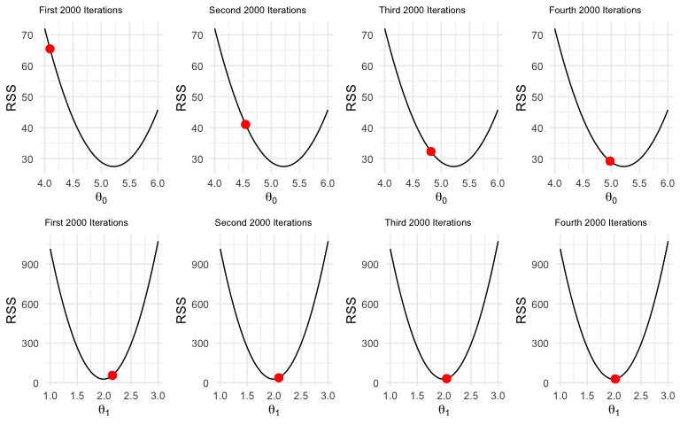
Recall we started with $\theta_0 = 3$. You can see after the first 2000 iterations, its value is just over 4. After the fourth set of iterations, its near the minimum. For $\theta_1$, it’s hard to notice the change. Its initial value was zero but after the first 2000 iterations, it had already overshot the minimum and then very slowly moved into place.

Comparing the Three Methods

A few more iterations

After 8000 iterations, we still haven’t reached the minimum. Let’s do another 20,000 iterations, then compare the results to lm and optim.

thetas <- gradient_descent(thetas, rate=0.001, iter=20000)

data.frame(
  lm = lm_thetas,
  optim = optim_thetas,
  gradient_descent = thetas,
  row.names = c("theta_0", "theta_1")
) %>%
  t() %>%
  as.data.frame()

output:

                  theta_0  theta_1
lm               5.218865 1.985435
optim            5.218865 1.985435
gradient_descent 5.217459 1.985644

Our rudimentary gradient_descent function does pretty well. Incidentally, it would take another 30,000 iterations at the 0.001 learning rate to achieve the same results as lm and optim to 6 decimal places.

To reduce the number of steps required, we could try to optimize the gradient_descent function by making the learning rate adaptive. A larger learning rate allows for a faster descent but will have the tendency to overshoot the minimum and then have to work its way back down from the other side. Meanwhile, a learning rate too small means a slower descent but less bouncing around the minimum on approach. So if we could dynamically adapt the learning rate, we could conceivably get closer to the minimum with less iterations.

Optimization Methods

When using machine learning models, you won’t really need to care about how they optimize. In fact, most of the time you won’t be able to change the optimization method. As an aside, R’s lm function doesn’t use numerical optimization. It uses linear algebra to solve the equation $X\beta=y$, using QR factorization for numerical stability, as detailed in A Deep Dive Into How R Fits a Linear Model.

R’s optim function is a general-purpose optimization function that implements several methods for numerical optimization. We used it earlier to estimate $\theta_0$ and $\theta_1$ to compare it with our gradient descent solution. You can specify one of many methods to use for optimization. I used "BFGS" in order to demonstrate the use of the gradient function.

The Python SciPy package has the scipy.optimize.minimize function for minimization using several numerical optimization methods, including Nelder-Mead, CG, BFGS and many more.

Nelder & Mead

From the R documentation,

The default method is an implementation of that of Nelder and Mead (1965), that uses only function values and is robust but relatively slow. It will work reasonably well for non-differentiable functions.

If your function is not differentiable, you can start with this method. From a computational perspective, if you do not have a lot of data, this method may be sufficient.

BFGS

BFGS is a popular method used for numerical optimization. It is one of several methods that can make use of a gradient function that returns a gradient vector that specifies the direction that $\theta$ should move for the fastest descent towards the minimum. BFGS is one of the default methods for SciPy’s minimize. According to the SciPy documentation,

method : str or callable, optional

If not given, chosen to be one of BFGS, L-BFGS-B, SLSQP, depending if the problem has constraints or bounds.

L-BFGS-B

A modified version of BFGS. The “L” stands for limited memory and as as the name suggests, can be used to approximate BFGS under memory constraints. The “B” stands for box constraints which allows you to specify upper and lower bounds so you’d need to have some idea of where your parameters should lie in the first place.

And so many more…

An exhaustive list of the various optimization methods is beyond the scope of this article. Knowing which method is best to use will require some research and probably some domain knowledge of your data. For machine learning, you will rarely need to be concerned about this but for few models such as Scikit Learn’s sklearn.linear_model.Ridge – which, by default, will auto-select a method (which it calls a “solver”) based on the type of data.

Final Words

Supervised machine learning is an optimization problem in which we are seeking to minimize some cost function, usually by some numerical optimization method. The fundamentals of the optimization process are well explained with gradient descent but in practice, more sophisticated methods such as stochastic gradient descent and BFGS are used. Thankfully, you’ll rarely need to know the gory details in practice.

Keep in mind that I’ve only described the optimization process at a fairly rudimentary level. There are nuances that I’ve omitted. For example, what happens when we have more complicated cost functions and the parameter space has more than one global minimum, i.e. many local minima?

Finally, it’s worth noting that the optimization process in artificial neural networks (ANN), while based on the same idea of minimizing a cost function, is a bit more involved. ANNs tend to have many layers, each with a set of associated parameters called weights and biases. Adjusting all the weights and biases at the various layers is done through a process called back propagation, a topic for another day.

Hope you enjoyed this post!