If you’re new to the world of R Studio, wrapping your head around R Markdown notebooks and documents can be a little tricky. Notebooks are meant to be interactive and are great for mixing markdown with R code blocks as you work your way through a report. Then you try to print and… not what you expected. So, what’s going on under the hood and how do you fix it?

Markdown Notebooks vs. Documents

Despite what you may read, there’s not much difference between the two. Conceptually, if you wanted to quickly jot something down in a notebook, you’d just open it and start writing whereas if you were about to write a report you’d be thinking about fonts, styles, layout and the such.

So, if you create a notebook, you don’t specify any additional options; R Studio will immediately open a new document with a defaut template and off you go, whereas if you create a document, you’d need to select a few options before proceeding.

But, it’s the same! In the end, you end up with an .Rmd document with some metadata in the YAML header at the top, like this

---
title: "Untitled"
output: html_document
---

If you select a document template, you may see some additional YAML depending on the specific template, such as author and abstract entries, for example, (which I do not show for simplicity). Since I created an R Document that outputs in HTML, the output type is html_document. An R Notebook would have had output: html_notebook instead. Want both?

---
title: "Untitled"
output:
  html_document: default
  html_notebook: default
---

When there is more than one output type, each type will appear in a separate, indented line. default means to use default settings for each output type.

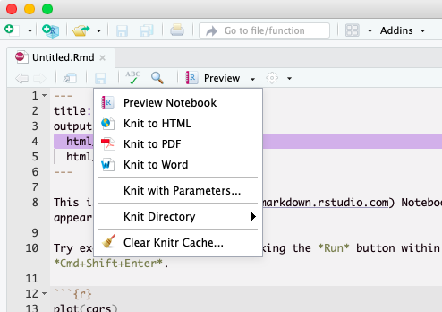
After saving this file with the additional output line, R Studio will update its Output dropdown menu to include a Preview Notebook option.

It’s typical for a notebook to contain a mix of markdown text and code blocks like this:

---
title: "R Notebook"
output:
  html_document: default
  html_notebook: default
---

Welcome to my **cool** notebook!

```{r}
qnorm(0.975)
```

For a 5% significance level, \$$z^* = 1.960\\$

Printing your HTML Output

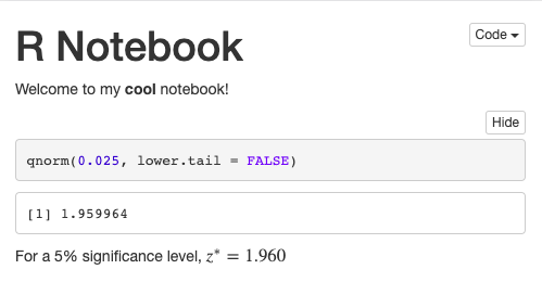
If you preview your Notebook, it should look something like this:

But… if you try to print it, it would look more like this:

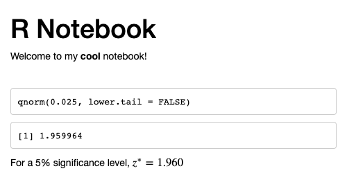
Note a couple of differences:

• The printed version is black & white
• The code box background colour is gone

These are just two differences that can be seen with this small notebook but there are more. For example, quoted text using markdown such as > some quoted text is completely different. Give it a try.

HTML vs. PDF

Converting your R Markdown to an output form for viewer consumption is a process known in R as knitting. Options include Knit to HTML and Knit to PDF. You may also see other Knit to… options such as Knit to Word and others can be added, such as Knit to Powerpoint, though I won’t go further into those.

HTML

Notebooks are written using Markdown, a lightweight markup language originally designed to be output as HTML, so it’s no wonder that this is one of R Studio’s Knit to options. The HTML is then formatted with CSS using one of the most ubiquitous CSS libraries for web design, Bootstrap. The differences between HTML screen and print output is controlled by Bootstrap’s CSS media queries. One way to tweak this CSS to your liking is to customize the output options in the YAML header.

One way of doing this is to add a reference to a CSS file. Let’s say you create a file called styles.css in the same directory as your .Rmd notebook file. You can then reference it like this:

---
title: "R Notebook"
output:
  html_document:
    css: styles.css
  html_notebook: default
---

You can now override some CSS styles in your styles.css file to make the screen and print output more synchronized.

@media print, screen {
  h1.title {
    font-size: 2.4em;
  }

  h2 {
    font-size: 1.6em;
  }

  blockquote {
    font-size: 0.8em;
    border: 0;
    border-left: 5px solid #ccc;
  }

  pre.r {
    background-color: #f5f5f5 !important;
  }
}

Unfortunately, one Bootstrap style that can’t be overriden is the black (& white) print style. This is due to the way Bootstrap defines this style. Bootstrap 3 is embedded in the rmarkdown package. In the bootstrap.css file you can find the responsible style.

  ⫶
@media print {
  *,
  *:before,
  *:after {
    color: #000 !important; /* set all text to black */
    text-shadow: none !important;
    background: transparent !important;
    -webkit-box-shadow: none !important;
            box-shadow: none !important;
  }
  ⫶
}

This is a CSS problem! There is no way to remove a style by overriding it. You could change the colour to something other than black but this still overrides all other style colours. What we really need is to remove that setting so that individual styles can control their own colour. You’d need to remove this line from the package but this is a hack and it would be “reset” when the package gets updated.

PDF

Knit to PDF creates a PDF file with a completely different format. The name is somewhat misleading as it’s not the only knit option that produces PDF output. It’s more like the vanilla PDF output.

It turns out that to produce PDF documents, R Studio uses pandoc, a document converter, which in turn uses a LaTeX package. There are options for customizing some output such as firgures, data frames and syntax highlighting, but if you want that “browser notebook” style, you should stick to HTML output. You can then convert that output to a PDF, if desired.

Of course, if you’re writing a book, dissertation, scientific paper, etc. you cannot avoid PDF output and getting your hands dirty. Check out the R Markdown Gallery to see some examples of PDF output. Then if you dare, check out the chapter PDF document of R Markdown: The Definitive Guide.

The End

Actually, this is just the beginning. You can use R Markdown to create presentations, dashboards, websites, books, journals, interactive tutorials, …

Go forth and markdown!